The fifth value, the dictionary, contains the critical values of the test-statistic at the 1, 5 and 10 percent values respectively. An alternative means of identifying a mean reverting time series is provided by the concept of stationaritywhich we will now discuss. A time series or stochastic process is defined to be strongly stationary if its joint probability distribution is invariant under translations in time or space.
Navigation menu
In particular, and of key importance for traders, the mean and variance of the process do not change over time or space and they each do not follow a trend. A critical feature of stationary price series is that the prices within the series diffuse from their initial value at a rate slower than that of a Geometric Brownian Motion. By measuring the rate of this diffusive behaviour we can identify the nature of the time series. We will now outline a calculation, namely the Hurst Exponent, which helps us to characterise the stationarity of a time series.
The goal of the Hurst Exponent is to provide us with a scalar value that will help us to identify within the limits of statistical estimation whether a series is mean reverting, random walking or trending. The idea behind the Hurst Exponent calculation is that we can use the variance of a log price series to assess the rate of diffusive behaviour.
The key insight is that if any autocorrelations exist i.
Mean reversion (finance)
In addition to characterisation of the time series the Hurst Exponent also describes the extent to which a series behaves in the manner categorised. To calculate the Hurst Exponent for the Google price series, as utilised above in the explanation of the ADF, we can use the following Python code:. In addition, we will consider the concept of cointegrationwhich will allow us to create our own mean reverting time series from multiple differing price series.
Finally, we will tie these statistical techniques together in order to form a basic mean reverting trading strategy. In statisticsregression toward or to the mean is the phenomenon that arises if a random variable is extreme on its first measurement but closer to the mean or average on its second measurement and if it is extreme on its second measurement but closer to the average on its first. The conditions under which regression toward the mean occurs depend on the way the term is mathematically defined.
The British polymath Sir Francis Galton first observed the phenomenon in the context of simple linear regression of data points. Galton [5] developed the following model: pellets fall through a quincunx to form a normal distribution centred directly under their entrance point. These pellets might then be released down into a second gallery corresponding to a second measurement.
Galton then asked the reverse question: "From where did these pellets come? The answer was not ' on average directly above '. Rather it was ' on average, more towards the middle 'for the simple reason that there were more pellets above it towards the middle that could wander left than there were in the left extreme that could wander to the right, inwards. As a less restrictive approach, regression towards the mean can be defined for any bivariate distribution with identical marginal distributions.
Two such definitions exist.
Harnessing The Power of Multi-Strategy Investing
Not all such bivariate distributions show regression towards the mean under this definition. However, all such bivariate distributions show regression towards the mean under the other definition. Jeremy Siegel uses the term "return to the mean" to describe a financial time series in which " returns can be very unstable in the short run but very stable in the long run.
Suppose that all students choose randomly on all questions. Then, each student's score would be a realization of one of a set of independent and identically distributed random variableswith an expected mean of Naturally, some students will score substantially above 50 and some substantially below 50 just by chance. Thus the mean of these students would "regress" all the way back to the mean of all students who took the original test.
No matter what a student scores on the original test, the best prediction of their score on the second test is If choosing answers to the test questions was not random — i. Most realistic situations fall between these two extremes: for example, one might consider exam scores as a combination of skill and luck.
In this case, the subset of students scoring above average would be composed of those who were skilled and had not especially bad luck, together with those who were unskilled, but were extremely lucky. On a retest of this subset, the unskilled will be unlikely to repeat their lucky break, while the skilled will have a second chance to have bad luck.
Cointegration
Hence, those who did well previously are unlikely to do quite as well in the second test even if the original cannot be replicated. The following is an example of this second kind of regression toward the mean. A class of students takes two editions of the same test on two successive days. It has frequently been observed that the worst performers on the first day will tend to improve their scores on the second day, and the best performers on the first day will tend to do worse on the second day. For the first test, some will be lucky, and score more than their ability, and some will be unlucky and score less than their ability.
Some of the lucky students on the first test will be lucky again on the second test, but more of them will have for them average or below average scores. Therefore, a student who was lucky on the first test is more likely to have a worse score on the second test than a better score. Similarly, students who score less than the mean on the first test will tend to see their scores increase on the second test.
If your favourite sports team won the championship last year, what does that mean for their chances for winning next season? To the extent this result is due to skill the team is in good condition, with a top coach, etc. But the greater the extent this is due to luck other teams embroiled in a drug scandal, favourable draw, draft picks turned out to be productive, etc. If one medical trial suggests that a particular drug or treatment is outperforming all other treatments for a condition, then in a second trial it is more likely that the outperforming drug or treatment will perform closer to the mean the next quarter.
If a business organisation has a highly profitable quarter, despite the underlying reasons for its performance being unchanged, it is likely to do less well the next quarter.
Click here to get a PDF of this post. There are many different types of trading strategies. Some traders trade with the trend buying high looking for higher highs or sell new low prices short looking for even lower lows in price, momentum strategies just look for a strong move to go a little farther, others trade a market inside a price range of support and resistance. What this article is going to talk about is the specific strategy of mean reversion, this is looking at prices as a kind of rubber band that stretches only so far and eventually snaps back to a historical long term average.
Mean reversion trading strategies consist of signals that bet on extended prices eventually snapping back from overbought or oversold conditions and reverting back to the mean of historical pricing. It is a trade that takes a position on a quantifiable technical signal that price has moved too far and too fast in one direction and the probabilities that it will return to an average are high.
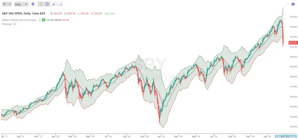
One simple way to look for a reversion to the mean trade signal is by setting visual deviations around prices using technical indicators like Bollinger Bands or Keltner Channels that usually measure the distance from the day moving in standard deviations of price. When a market drops dramatically or rises parabolically three or four deviations from the day moving average the odds are that it will revert back to that average in days or weeks the majority of time.
Of course this does not always happen as markets rotate from ranges to trends, and can go farther than anyone thought possible so you must always use a stop loss for the times when a trend continues and does not revert. One strategy is to buy dips to the lower 3rd standard deviation Keltner Channel or sell rallies short to the upper 3rd standard deviation Keltner Channel and set a stop loss if price closes back outside your entry channel signal.
Your profit target could be back to the day moving average.
A mean reversion entry is taking a trade that is at short term extreme prices that has a good chance of returning to more normal long term price metrics. Chart Courtesy of TrendSpider. This is not investment advice just one example and any trade you take should meet your own risk tolerance and return goals. What is the Uptick Rule?
Mean reversion excel. A Mean Reversion Strategy Explained
Share this:. Share 0. Our Partners. Chart Reading.
A reader sent me some trading rules he got from a newsletter from Nick Radge. He wanted to know if these rules really did as well as published in the newsletter. They seemed too simple to produce such good results. This is a basic mean reversion or pullback strategy. The strategy as presented was long and short and went on margin but he wanted to know how it did the long only since he did not short. Subscribe to my newsletter to receive updates and tips on trading and get instant access to Market Regimes as I use them in my trading.
No fancy rules are here. It is standard mean reversion strategy. At times the strategy will produce more signals than there are open slots for. To trade this, one must be watching the markets during the day and take the signals as they happen. This is not realistic for most people since they are not full time traders sitting in front of their computers. One could automate this, but that is not a simple task. The first time I heard about this rule and tested. I thought there is no way this rule could work. I figured it would destroy a perfectly good strategy. I was flabbergasted that it worked and produced good results.
This is why I say that one should test ideas before throwing them out. You never know what will work. When there are more signals than open positions, the code would randomly choose which stocks to enter. I then ran runs for each test. Surprisingly good results from such simple rules. The results are not as good as using the Russell but still good. Probably because of the smaller universe which leads to lower exposure. The spreadsheet includes the full Monte Carlo run data. In the spreadsheet are details on how to obtain the AmiBroker code that I used for this post. What I like about this strategy is how simple it is, yet produces good results.